Uptrace: Querying Metrics

TIP

To learn about metrics, see OpenTelemetry Metricsopen in new window documentation.

Uptrace provides a powerful query language that supports joining, grouping, and aggregating multiple metrics in a single query.

Uptrace aims to be compatible with the Prometheus query language while extending it in a meaningful way. If you're already familiar with PromQL, read this to learn how Uptrace is different .

Writing queries

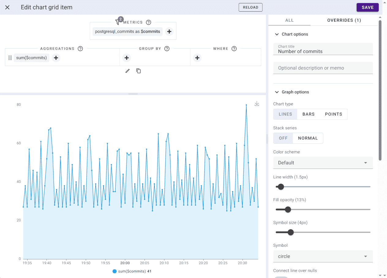
Uptrace allows you to create dashboards using UI or YAML configuration files. This documentation uses the more compact YAML format, but you can achieve the same with the UI.

YAML:

metrics:
  - postgresql_backends as $backends

query:
  - $backends

UI:

Grid item form

You can find the existing dashboard templates on GitHubopen in new window.

Aliases

Because metric names can be quite long, Uptrace requires you to provide a short metric alias that must start with the dollar sign:

metrics:
  # metric aliases always start with the dollar sign
  - system_filesystem_usage as $fs_usage
  - system_network_packets as $packets

You must then use the alias instead of the metric name when writing queries:

query:
  - sum($fs_usage)

Uptrace also allows to specify an alias for expressions:

query:
  - $fs_usage{state="used"} as used_space
  - $fs_usage{host_name='host1', device='/dev/sdd1'} as host1_sdd1

You can then reference the expression using the alias:

metrics:
  - service_cache_redis as $redis
query:
  - $redis{type="hits"} as hits
  - $redis{type="misses"} as misses
  - hits / (hits + misses) as hit_rate

Grouping

Uptrace allows to customize grouping on the metric and function level:

$metric by (attr1, attr2)
sum($metric by (attr1, attr2))
avg(sum($metric by (attr1, attr2)) by (attr1))

You can also specify grouping for the whole expression:

$metric1 by (type) / $metric2 group by host_name

# The same.
$metric1 by (type, host_name) / $metric2 by (host_name)

And for the whole query affecting all expressions:

$metric1 | metric2 | group by host_name

# The same using expression-wide grouping.
$metric1 group by host_name | $metric2 group by host_name
# Or custom grouping.
$metric1 by (host_name) | $metric2 by (host_name)

Manipulating attributes

You can rename attributes like this:

$metric1 by (deployment_environment as env, service_name as service)
$metric1 | group by deployment_environment as env, service_name as service

To manipulate attribute values, you can use replace and replace_regexp functions:

group by replace(host_name, 'uptrace-prod-', '') as host
group by replace_regexp(host, `^`, 'prefix ') as host
group by replace_regexp(host, `$`, ' suffix') as host

To change strings case, use upper and lower functions:

group by lower(host_name) as host
group by upper(host_name) as host

You can also use a regexp to extract a substring from the attribute value:

group by extract(host_name, `^uptrace-prod-(\w+)$`) as host

Filtering

Uptrace supports all the same filters just like PromQL:

node_cpu_seconds_total{cpu="0",mode="idle"}
node_cpu_seconds_total{cpu!="0",mode=~"user|system"}

In addition, you can also add global filters that affect all expressions:

$metric1 | $metric2 | where host = "myhost" | where service = "myservice"

# The same.
$metric1{host="myhost",service="myservice"} | $metric2{host="myhost",service="myservice"}

Global filters support the following operators:

=, !=, <, <=, >, >=, for example, where host_name = "myhost".
~, !~, for example, where host_name ~ "^prod-[a-z]+-[0-9]+$".
like, not like, for example, where host_name like "prod-%".
in, not in, for example, where host_name in ("host1", "host2").

Joining

Uptrace supports math between series, for example, to add all equally-labelled series from both sides:

$mem_free + $mem_cached group by host_name, service_name

# The same.
$mem_free by (host_name, service_name) + $mem_cached by (host_name, service_name)

Uptrace also automatically supports one-to-many/many-to-one joins:

# One-to-many
$metric by (type) / $metric by (service_name, type)

# Many-to-one
$metric by (service_name, type) / $metric by (type)

You can rename attributes like this:

$metric by (foo as baz) + $metric by (bar as baz)

Supported functions

Like Prometheus, Uptrace supports 3 different types of functions: aggregate, rollup, and transform.

Aggregate functions combine multiple timeseries using the specified function and grouping attributes. When possible, aggregation is pushed down to ClickHouse for maximum efficiency.

min
max
sum
avg
median, p50, p75, p90, p99, count. Only histograms.

The count function returns the number of observed values in a histogram. To count the number of timeseries, use uniq($metric, attr1, attr2), which efficiently counts the number of timeseries directly in ClickHouse.

Rollup (or range/window) functions calculate rollups over data points in the specified lookbehind window. The number of timeseries remains the same.

min_over_time, max_over_time, sum_over_time, avg_over_time, median_over_time
rate and irate
increase and delta

Transform functions operate on each point of each timeseries. The number of timeseries remains the same.

abs
ceil, floor, trunc
cos, cosh, acos, acosh
sin, sinh, asin, asinh
tan, tanh, atan, atanh
exp, exp2
ln, log, log2, log10
per_sec divides each point by the number of seconds in the grouping interval. You can achieve the same with $metric / _seconds.
per_min divides each point by the number of minutes in the grouping interval. You can achieve the same with $metric / _minutes.

Additionally, grouping functions manipulate attributes and can only be used in grouping expressions:

lower(attribute) lowers the case of the attribute value.
upper(attribute) uppers the case of the attribute value.
extract(haystack, pattern) extracts a fragment of the haystack string using the regular expression pattern.
replace(haystack, substring, replacement) replaces all occurrences of the substring in haystack by the replacement string.
replace_regexp(haystack, pattern, replacement) replaces all occurrences of the substring matching the regular expression pattern in haystack by the replacement string.

If Uptrace does not support the function you need, please open an issueopen in new window on GitHub.

Offset

The offset modifier allows to set time offset for a query.

For example, this query retrieves the value of http_requests_total from 5 minutes ago, relative to the query evaluation time:

http_requests_total offset 5m

A negative offset allows to look ahead of the query evaluation time:

http_requests_total offset -5m

Instruments

OpenTelemetry offers various instrumentsopen in new window, each with its own set of aggregate functions:

Instrument Name	Timeseries kind
Counteropen in new window, CounterObserveropen in new window	Counter
UpDownCounteropen in new window, UpDownCounterObserveropen in new window	Additive
GaugeObserveropen in new window	Gauge
Histogramopen in new window	Histogram
AWS CloudWatch	Summary

Counter

Counter is a timeseries kind that measures additive non-decreasing values, for example, the total number of:

processed requests
received bytes
disk reads

Uptrace supports the following functions to aggregate counter timeseries:

Expression	Result timeseries
`$metric`	Sum of timeseries
`per_min($metric)`	`$metric / _minutes`
`per_sec($metric)`	`$metric / _seconds`

Gauge

Gauge is a timeseries kind that measures non-additive values for which sum does not produce a meaningful correct result, for example:

error rate
memory utilization
cache hit rate

Uptrace supports the following functions to aggregate gauge timeseries:

Expression	Result timeseries
`$metric`	Avg of timeseries
`avg($metric)`	Avg of timeseries
`min($metric)`	Min of timeseries
`max($metric)`	Max of timeseries
`sum($metric)`	Sum of timeseries
`per_min($metric)`	`$metric / _minutes`
`per_sec($metric)`	`$metric / _seconds`
`delta($metric)`	Diff between curr and previous values

* Note that the sum, per_min, per_sec, and delta functions should not be normally used with this instrument and were added only for compatibility with Prometheus and AWS metrics. For the same reason, per_min(sum($metric)) and delta(sum($metric)) are also supported.

Additive

Additive is a timeseries kind which measures additive values that increase or decrease with time, for example, the number of:

active requests
open connections
memory in use (megabytes)

Uptrace supports the following functions to aggregate additive timeseries:

Expression	Result timeseries
`$metric`	Sum of timeseries
`sum($metric)`	Same as `$metric`
`avg($metric)`	Avg of timeseries
`min($metric)`	Min of timeseries
`max($metric)`	Max of timeseries
`per_min($metric)`	`$metric / _minutes`
`per_sec($metric)`	`$metric / _seconds`
`delta($metric)`	Diff between curr and previous values

* Note that the delta function should not be normally used with this instrument and was added only for compatibility with Prometheus and AWS metrics.

Histogram

Histogram is a timeseries kind that contains a histogram from recorded values, for example:

request latency
request size

Uptrace supports the following functions to aggregate histogram timeseries:

Expression	Result timeseries
`count($metric)`	Number of observed values in timeseries
`p50($metric)`	P50 of timeseries
`p75($metric)`	P75 of timeseries
`p90($metric)`	P90 of timeseries
`p95($metric)`	P95 of timeseries
`p99($metric)`	P99 of timeseries
`avg($metric)`	`sum($metric) / count($metric)`
`min($metric)`	Min observed value in the histogram
`max($metric)`	Max observed value in the histogram

Note that you can also use per_min(count($metric)) and per_sec(count($metric)).

Summary

Sum is a timeseries kind that exists for compatibility with Prometheus and AWS Cloud Watch. It stores the min, max, sum, and count aggregates of observed values.

Expression	Result timeseries
`sum($metric)`	Sum of timeseries
`count($metric)`	Number of observed values in timeseries
`avg($metric)`	`sum($metric) / count($metric)`
`min($metric)`	Min observed value
`max($metric)`	Max observed value

Note that you can also use per_min(count($metric)) and per_sec(count($metric)).

Misc

What are timeseries?

A timeseries is a metric with an unique set of attributes, for example, each host has a separate timeseries for the same metric name:

# metric_name{ attr1, attr2... }
system_filesystem_usage{host_name='host1'} # timeseries 1
system_filesystem_usage{host_name='host2'} # timeseries 2

You can add more attributes to create more detailed and rich timeseries, for example, you can use state attribute to report the number of free and used bytes in a filesystem:

system_filesystem_usage{host_name='host1', state='free'} # timeseries 1
system_filesystem_usage{host_name='host1', state='used'} # timeseries 2

system_filesystem_usage{host_name='host2', state='free'} # timeseries 3
system_filesystem_usage{host_name='host2', state='used'} # timeseries 4

With just 2 attributes, you can write a number of useful queries:

# the filesystem size (free+used bytes) on each host
query:
  - sum($fs_usage) group by host_name

# the number of free bytes on each host
query:
  - sum($fs_usage{state='free'}) as free group by host_name

# fs utilization on each host
query:
  - sum($fs_usage{state='used'}) / sum($fs_usage) as fs_util group by host_name

# the size of your dataset on all hosts
query:
  - sum($fs_usage{state='used'}) as dataset_size

Binary operator precedence

The following list shows the precedence of binary operators in Uptrace, from highest to lowest.

^
*, /, %
+, -
==, !=, <=, <, >=, >
and, unless
or

Operators on the same precedence level are left-associative. For example, 2 * 3 % 2 is equivalent to (2 * 3) % 2.

Uptrace: Querying Metrics

# Writing queries

# Aliases

# Grouping

# Manipulating attributes

# Filtering

# Joining

# Supported functions

# Offset

# Instruments

# Counter

# Gauge

# Additive

# Histogram

# Summary

# Misc

# What are timeseries?

# Binary operator precedence

# See also